Multi-Armed Bandit
MAB report案例 Multi-Armed Bandit. Assuming there are multiple “arms” you can pull, and each arm will give a return or loss back to you.
MAB report
1. Introduction
Slot machines are the most common equipment in casinos. Assuming there are multiple “arms” you can pull, and each arm will give a return or loss back to you. The goal of this problem is to maximize the total returns. In this report, four most used methods were implemented to solve this typical reinforcement learning problem – Multi-Armed Bandit (MAB). We have no idea about the hidden distributions of returns of each arm, also the resources and time constrain us to balance the “exploring” and “exploiting”.
2. Methods MAB report案例
2.1 Greedy
The most simple and intuitive action is greedy. The model tries to compute the return of each arm, which means each arm has to be pulled as least once. Then just keep pulling the arm with the most return. Obviously, greedy method abandons the opportunity to explore other better arms, and it is easily to be influenced by the result of first experiment.
2.2 Epsilon-greedy MAB report案例
Epsilon-greedy algorithm improves the shortage of greedy method. During each round, the probability that the play chooses to pull the arm that yield highest payouts in the past is 1-ε (the probability of exploitation), and the probability to randomly choose an arm is ε (the probability of exploration).
2.3 Thompson Sampling
Thompson Sampling algorithm is a posterior sampling, which applies Bayesian rules. Let’s take the example of Beta-Bernoulli Bandit to illustrate the logic behind Thompson Sampling Algorithm. Assume there are K arms and each arm has the probability θκ to return 1 and probability 1–θκ to return 0. The mean reward θ=(θ₁,θ₂,···,θκ ) is unknown, thus a prior distribution of θ has been assumed – Beta distribution with parameters α=(α₁,α₂,···,ακ) and β=(β₁,β₂,···, βκ) .
As observations gathers, the parameters are updated via Bayesian rule. The success probability estimate θκ is randomly sampled from the posterior distribution. Which assures the action is optimal, conditioned on history observations. Thus, compared to the Greedy algorithm and Epsilon-greedy algorithm. The Thompson Sampling will explore to find the optimal arm while avoid wasting chance to explore the arm which would not be helpful.
2.4Upper Confidence Bound MAB report案例
The Upper Confidence Bound (UCB) can make decisions to explore that are driven by the confidence in the estimated value of the arms that have been selected. The Epsilon-greedy tends to be gullible since it is easily misled by a few negative returns. Instead, UCB avoids misleading by keeping track of confidences of the estimated value of all of the arms.
3. Experiments
In this section, some simulations and explorations were done.
3.1Simulations for Greedy and Epsilon-greedy Algorithms
First, generate optimal arms randomly by standard normal distribution, and for each round, we generate the reward data randomly too for each optimal arm. Then play 500 rounds with 10 arms, assume the distribution of rewards is standard normal and set the epsilon to be 0.1 and 0.01. Define probs follows U [0,1] with 500 numbers. During each round, if probs[i] is less than epsilon, then randomly sample an arm from all arms, otherwise, choose to pull the arm with best rewards so far.
Now we do the simulation under the scenario:
play 500 rounds with 10 arms under the epsilon be 0, 0.1 and 0.01, separately.
 1
1 We found the epsilon 0.1 strategy has the best average rewards and move to the optimal arm more quickly than the others. Thus, we believe that 0.1 might be a good balance of probability between exploration and exploitation.MAB report案例
3.2 Bandits have normally distributed rewards with small variance
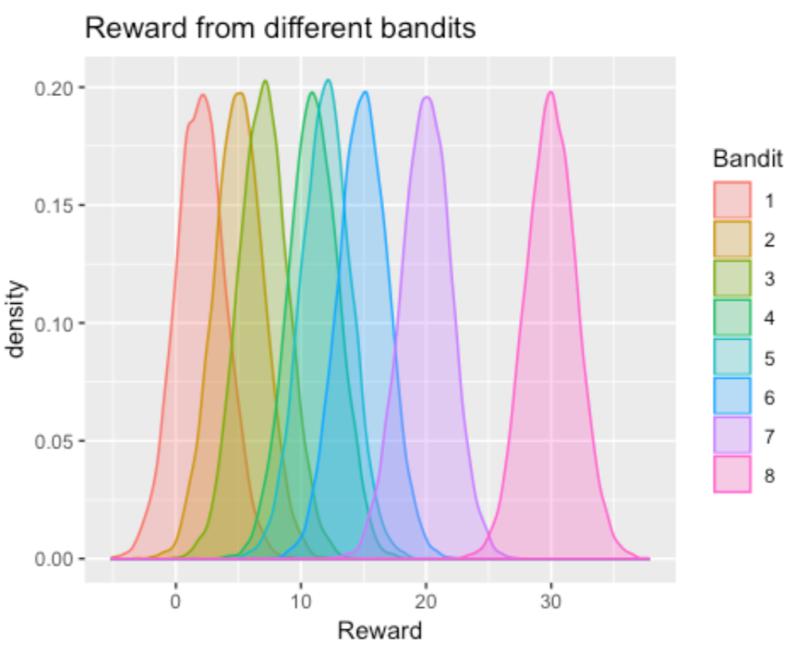
First of all, we randomly set the true mean rewards randomly for 8 machines to be (2, 5, 7, 11, 12, 15, 20, 30). Note that the numbers are just randomly chosen, people can choose any combinations of numbers they want. For each machine, we randomly generated normal distribution with mean equaling to the true mean, and the standard deviation equaling to 2, which is small. Then generate simulation data and plot these distributions.
 2
2 The plot is just a visualization of the distributions that we designed for each arm.
3.3 Thompson Sampling Algorithm
First, define a function rnormgamma, which returns a dataframe with random gamma distribution and normal distribution with the parameters people define. Then construct the Thompson Sampling function TS by inputting the number of plays, the observed reward data, the parameters of those two distributions mentioned above.
Define the prior distribution and likelihood based on reward data and assumptions, then updated the αι by adding 1 if the ith arm gets a reward 1 and update the βι by adding 1 if the ith arm gets 0 reward. Finally, the function returns a list of total reward, the bandit selected, the number of plays and the sums of rewards of each arm.
If we use normal-gamma prior and normal likelihood to estimate posterior distribution, with 1000 plays, simulated data and the true mean being 30, we found the final total reward is 28775.88, and selected bandits quickly converge to the 8th bandit, whose accumulated reward is 28140.73115.MAB report案例
3.4 Upper Confidence Bound Algorithm
Like the explanation above, in the UCB function, the upper confidence bound is computed for each arm, and then iteratively update the highest bound to be the max upper bound. If we play 1000 rounds and generate the simulated reward data, we found the final total reward is 29936.02, and selected bandits converge even more quickly than Thompson Sampling to the 8th bandit, whose accumulated reward is 29874.60. The Thompson Sampling tried other suboptimal or worse bandits a bit before finding the best one.
3.5 Bandits have rewards with different distributions
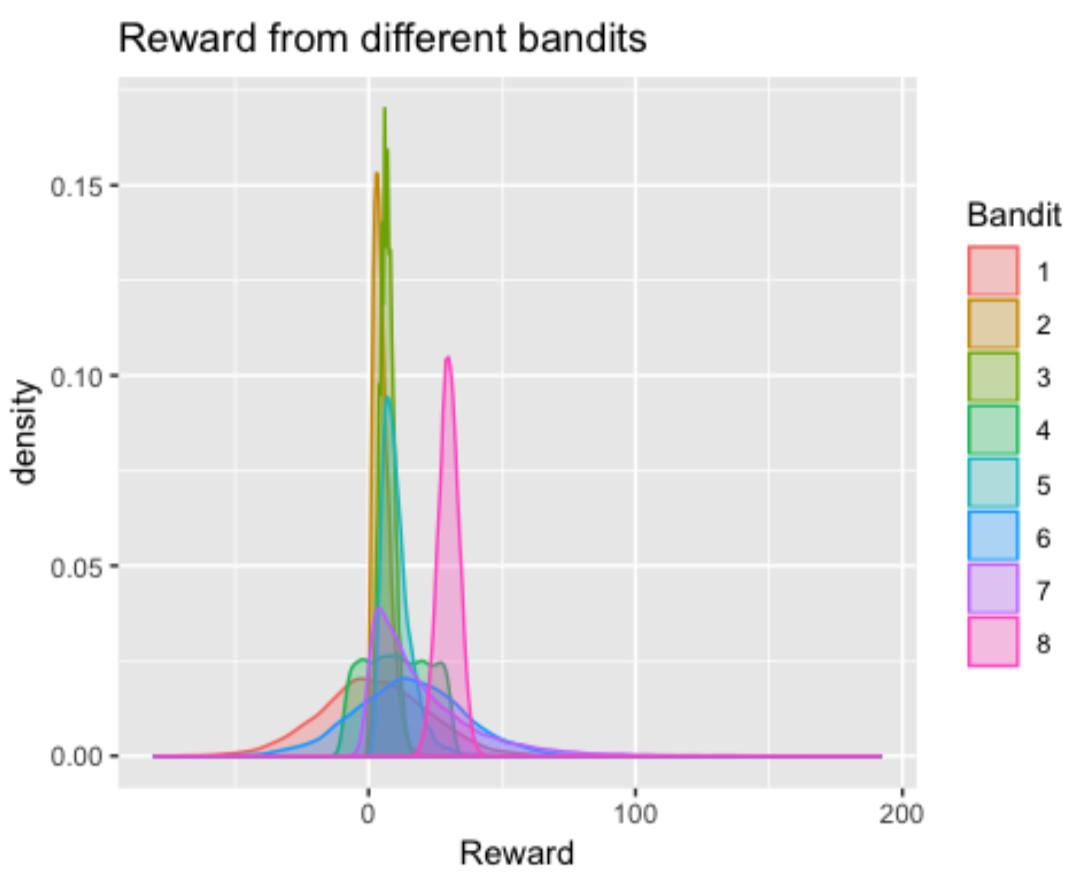
Let’s set the mean to be the same as the beginning, while all 8 arms have different distributions: Normal, Gamma, Poisson, Uniform, Log-normal, Exponential and Binomial. Then generate the simulated data whose plot like below:
 MAB report代写
 The plot is just a visualization of the distributions that we designed for each arm.
If we conduct UCB on rewards with different distributions in the same way and play 1000 rounds, the total reward is 29675.67, and selected bandits converge a little bit slower than the previous UCB experiment.
If we conduct Thompson Sampling on rewards with different distributions in the same way and play 1000 rounds, the total reward is 28664.25, and selected bandits converge to the optimal arm almost at the same speed as the previous Thompson Sampling experiment.
In a word, even though we simulate different data with different assumptions, the conclusions seem to be the same.
3.6 Using MCMC to estimate the posterior MAB report案例
To use the methods above, one must use conjugate priors of the likelihood in order to update posterior distributions in a straight forward way. However, if the appropriate conjugate priors do not exist, or we want to construct hierarchical models which include other variables that might influence the rewards. Thus, posterior distributions of the reward could not be estimated via the common way. Instead, MCMC could be used to estimate it.
MCMC tries to sample from posterior distribution by constructing a Markov Chain. With sufficient samples and applying other control measures (such as thinning and burn in), these samples drawn from the Markov Chain will approximate the posterior.
We use a function BUGS in the package “R2OpenBUGS” to summarize inferences and convergence in a table, then save the simulations in arrays.
4. More MAB report案例
The Bayesian solution begins by assuming priors on the probability of winning for each bandit. Hierarchical models will partially pool the bandits. For example, we may consider pulling different bandits within different casinos. Which include a region variable that may affect the rewards of bandits.
The bandits-within-casino structure implies the problem is hierarchical. Since each bandit may perform differently depending on which casino it locates. We allow the rewards rate to vary by using casino-specific attribute importance parameters.
更多其他: 案例 C++案例 CS案例 code案例 CS案例 cs案例 C语言案例 Data Analysis案例
